
Abstract
The induction machine is widely used in industrial fields due to its robustness, low cost, and good standardization. Indeed, its use in high-performance variable-speed drive systems requires the imposition of specific and complex control structures based on the mathematical model of the machine and its power supply. However, this chapter book deals with indirect stator field-oriented control (ISFOC) of an induction motor drive (IM), without a speed sensor. In previous works, the MRAS scheme has been used to estimate the speed and the rotor resistance. The reference model and the adjustable one, which are developed in the stationary stator reference frame, are used to estimate simultaneously the rotor speed and the rotor resistance (IM) from the knowledge of the stator currents and voltages. Simulation and experimental results are presented to validate the mathematical study as well as to prove the effectiveness and the robustness of the proposed scheme of control and sensorless ISFOC induction motor drive.
Keywords
- induction machine
- stator flux orientation model
- model reference adaptive system (MRAS)
- rotor speed
- resistance estimation
1. Introduction
The induction motor IM has long been used mainly at a constant speed. Its control remains a challenge for researchers, in order to optimize and control the motor in variable-speed drives. With advances in power electronics such as the appearance of GTO thyristors and subsequently IGBT transistors as well as digital electronics such as the development of new DSPs (Digital Signal Processors), the drive problem at variable speed is resolved and the control strategies have been implemented under satisfactory conditions.
The vector control (FOC: Field-Oriented Control) also called flux orientation control, it allows to reduce the behavior of the IM to that of a direct current DC motor (with separate excitation) to have the same performance in torque and speed [1, 2]. The FOC has very good accuracy for torque and speed. Moreover, this strategy, although sophisticated, has the disadvantage of requiring the installation of a mechanical sensor on the shaft of the motor and also has a high sensitivity to the parametric variations of the IM in particular to the rotor resistance [3]. Two methods are possible for flux-oriented vector control [4]. The first is called the Direct Control Method (DFOC) and the second is called Indirect Method (IFOC). This strategy consists of not estimating the flux but directly using the amplitude of its reference value ϕ*.
To address the problem of the presence of a speed sensor in the IFOC, we opt for a control without a mechanical sensor, which is based on the design of software sensors for the estimation of physical variables, such as the speed and rotor resistance. The design of such sensors is mainly based on the synthesis of observers or adaptive methods allowing parametric identification and sensorless control of the IM. In the literature, several methods of simultaneous estimation of speed and rotor resistance in sensorless IM drive have appeared. Among the most used techniques, we can mention:
Rotor resistance estimation using the transient state under the speed sensorless control of the induction motor [5].
Speed sensorless of IM drive with online model parameter tuning for steady-state accuracy [6, 7].
Simultaneous estimation of the rotor speed and the rotor resistance was estimated by adding a small alternating current to the rotor flux [8].
This chapter book presents a modeling and control of an asynchronous machine with and without mechanical sensors. However, the measurement of the currents and voltages will be used in order to estimate the speed and the rotor resistance using the Model Reference Adaptive System (MRAS) scheme. A theoretical study is given with detailed mathematical equations and accompanied by simulation and experimental results in order to demonstrate the effectiveness of the proposed method.
This chapter book is organized as follows. Section 2 presents an asynchronous motor model. While, in Section 3, an induction motor state model will be introduced. Section 4 formulates the stator field orientation control of the induction motor drive. Then, the simultaneous estimation of speed and rotor resistance will be illustrated and discussed in the section. Furthermore, the simultaneous estimation of speed and rotor resistance using MRAS technique. Simulation results are proposed in Section 6. Thereafter, in Section 7, we will present the experimental results obtained on a test bench provided with a chart of real-time control of the type dS1104. Finally, we ended up with a conclusion.
2. Asynchronous machine model
According to the laws of physics, the asynchronous machine can be associated with mathematical equations that involve its parameters. The implementation of these equations gives rise to the modeling. At the end of this operation, a problem arises; however, when the model is closest to reality, it becomes very complex and requires a very powerful and high-performance calculator. In order to simplify the calculation while keeping the most important phenomena and neglecting the secondary phenomena, and for the resulting model to be usable in both static and dynamic conditions, we must use simplifying assumptions.
2.1 Simplifying assumptions
The equations of the asynchronous machine are made by adopting the following simplifying assumptions [9, 10]:
The air gap is assumed to be constant, and the machine is symmetrical.
The current density is uniform in the conductor sections.
The magnetic circuit is unsaturated and perfectly laminated to the stator and to the rotor.
Winding resistances do not vary with temperature and skin and notch effects are neglected.
The spatial distribution of magnetomotor forces is assumed to be sinusoidal along the air gap.
The cage rotor is described as a balanced three-phase winding.
2.2 Mathematical model of the asynchronous machine
According to Figure 1, the Induction Motor (IM) has six windings:
The stator consists of three fixed windings (A,B,C) offset in the space of 120° from each other and crossed by three sinusoidal currents.
The rotor can be modeled by three identical windings and shorted (a,b,c) offset by 120° in space.
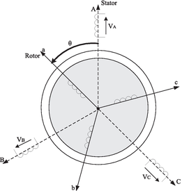
Figure 1.
Spatial representation of asynchronous machine windings.
2.2.1 Electrical equation
The Ohm law applied to the stator and rotor circuits is written in the following matrix form:
2.2.2 Magnetic equation
According to the simplifying assumptions, the relations between fluxes and currents are linear and can be written in the following matrix form:
We finally obtain the three-phase asynchronous model:
with:
2.2.3 Mechanical equation
The fundamental relationship of dynamics allows us to write:
2.3 Two-phase model of the machine
When studying transient phenomena, we are faced with the following problem:
The Eq. (6) of the matrix of mutual inductances being with nonconstant elements and the coefficients of the Eq. (8) are variable from where the analytical resolution of this system of equations becomes very difficult. To tackle this problem, we use mathematical transformations to describe the behavior of the machine using differential equations with constant coefficients, which facilitate its resolution. These transformations must preserve the instantaneous power and the reciprocity of mutual inductances.
The use of Park’s transformation makes it possible to circumvent these problems and simplify the statoric and rotoric equations in order to obtain a system of equations with constant coefficients, which considerably reduces the calculation time.
2.3.1 Park transformation
The transformation of Park makes it possible to go from a three-phase system abc to a two-phase system d and q axes. A Park P(β) matrix allows the passage of the Xabc quantities from the three-phase system to the two-phase Xdq quantities, rotating at a speed that depends on the stator or rotor quantities, such as (Figure 2).
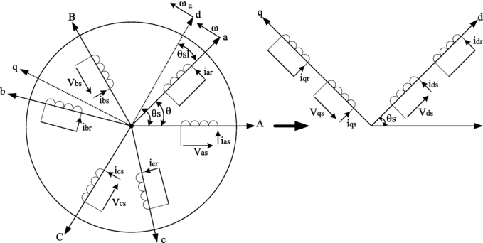
Figure 2.
Representation of the equivalent three-phase and two-phase asynchronous machine.
This matrix ensures the instantaneous power invariance and its calculation is obtained by taking
2.3.2 Electrical model of the asynchronous machine
By applying the Park transformation to the electric and magnetic equations of the asynchronous machine, we obtain the Eqs. (12) and (13), which are expressed in a reference frame running at an arbitrary speed ωa.
Stator equations.
Rotor equations.
with
For a balanced system, the stator and rotor homopolar components are zero. Knowing that the machine is caged and taking into account Eqs. (13), the Eqs. (11) and (12) are reduced to:
2.3.3 Electromagnetic couple expressions
We can see that the torque results from an interaction between flows and currents. The application of the transformation of Park provides us with several forms of expressions of the electromagnetic couple among which we distinguish:
The choice of the expression will depend on the type of fluxes orientation. In fact, we use (16) for the rotor orientation and (17) for the stator flux orientation.
3. Induction motor state model
The state model of an asynchronous machine allows the study of its transient states. Eq. (15), which forms the state equations of the machine, represents a nonlinear differential system with constant coefficients. (ωa = ωs and ωsl = ωs - ω).
The possibilities for choosing electrical state variables are diverse. This choice is characterized by the variables endowed with memory, such as the currents, the fluxes, the speed, and the angular position.
The machine state model is:
The quantities of the state vector are chosen according to the quantities to be controlled.
3.1 State model for stator flux orientation control
We consider the second expression of the electromagnetic couple given by Eq. (18).
The state variables used are ϕds, ϕqs, ids, and iqs. For this reason, we are interested to eliminate the flux ϕdr, ϕqr, and the current idr and iqr of the Eq. (15). This leads to a state representation of the asynchronous machine of the form:
with:
3.2 State model for rotor flux orientation control
We consider the second expression of the electromagnetic couple given by Eq. (18). The state variables used are ϕdr, ϕqr, ids, and iqs. For this reason, we are interested to eliminate the flux ϕds, ϕqs and the current idr and iqr of the Eq. (15). This leads to a state representation of the asynchronous machine of the form:
3.3 Simulation
The model of the asynchronous machine was tested by simulation with the Matlab-Simulink software. Figure 3(a) represents the curve of the speed during the direct start of the induction machine on the network with an application and cancelation of a load at time t = 0.4 s and at t = 0.7 s, respectively.
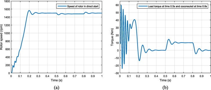
Figure 3.
Speed and torque of an asynchronous machine during a direct start.
The analysis of the previous results shows that the IM undergoes a very brutal transient state during its direct start on the network. The method for alleviating the various constraints consists in supplying the motor with a set of variable voltages in frequency and amplitude. Various approaches are possible and they are all based on the steady-state characteristics of the induction motor.
4. Stator field-oriented control of induction motor drive
Vector control offers a better solution to achieve better performance in variable-speed applications. This solution appeared with the work of Blaschke in early 1970. The vector control also called the flux orientation controller, consists in orienting the flux according to axis d, and therefore its component in axis quadrature q is zero in order to make the behavior of the asynchronous machine similar to that of a direct-current machine with independent excitation. The purpose of this control is to eliminate the coupling between the armature and the inductor, so that its operation is comparable to that of a direct-current machine, by breaking down the stator current into two components, one controlling the flow and the other controlling the torque. In our work, we will focus on the control by direction of the statoric flux.
By referring to a rotating reference frame, denoted by the superscript (d,q), the dynamic model of a three-phase induction motor can be expressed as follows [9, 10]:
with
The torque (Eq. (17)) looks like a DC machine if the second product is eliminated ϕqsIds. So, it is enough to orient the reference (d,q), so as to cancel the quadrature flux component, in other words, to orient the stator flux according to the axis d (ϕds = ϕs). Therefore, its quadrature component of axis q is zero (ϕqs = 0). In this case, the stator flux will be controlled by the d-axis stator current and the torque is controlled by the q-axis quadrature current. The new expression of the couple is:
Using Eq. (20), the
The reference
The IP speed controller is designed in order to stabilize the closed-loop sensorless speed control. The closed-loop transfer function is given by:
With:
The gains of the IP controller,
For
With:
Using the same method as the speed controller, the gains
In our simulation, we have used the time constant
4.1 Simulation results
Figure 4 represents the block diagram of the control by stator flux orientation of a 3 kW asynchronous machine with a mechanical sensor. It consists of a three-phase cage asynchronous machine powered by a pulse-width modulation (PWM) voltage inverter. A block for regulating the rotor speed with an IP corrector and that of the current with a PI corrector.
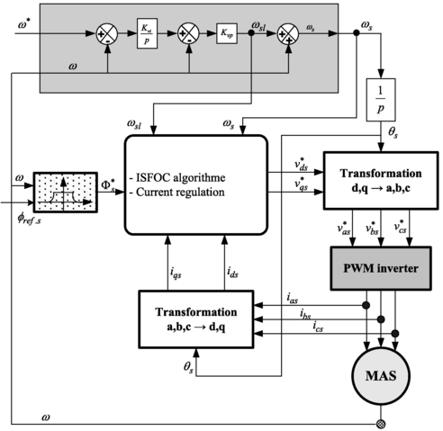
Figure 4.
Block diagram of the ISFOC of an asynchronous machine with speed sensor
The ISFOC of an asynchronous machine with a mechanical sensor was tested by simulation with the Matlab-Simulink software. In this study, we regulate the speed with an IP corrector (Kvi = 7.9665, Kvp = 0.3001) and the current by a PI corrector (Kip = 26.929, Kii = 7764.8). The set points are the stator flux and the speed.
4.1.1 Influence of load torque variation
In this part, we simulated the system for a speed setpoint of 1000 rpm at time 1 s, under the application of a load torque equal to 10 Nm between times t1 = 3 s and t2 = 5 s. We obtained the following results:
Figure 5(a) represents the curve of the speed during a load application at time t = 3 s and its cancelation at time t = 5 s, we can clearly see that the real speed is stable and converges toward its reference value, which shows the reliability of the proposed algorithm. Figure 5(b) shows the curve of the current ids and iqs. However, Figure 5(c) proves the orientation of the stator flux that we have chosen, so we notice that ϕds = ϕs and ϕqs = 0. Furthermore, Figure 5(d) shows that the curve of the electromagnetic torque and the quadratic current iqs are proportional, even during a load variation.
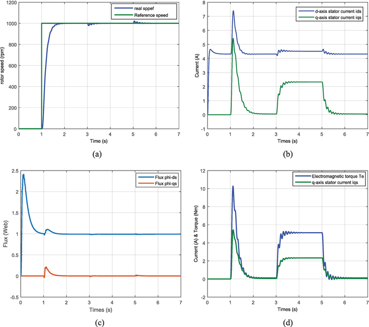
Figure 5.
Indirect stator flux-oriented controlled (ISFOC) induction motor drive under load torque.
4.1.2 Low-speed study and inversion of the direction of rotation
To increase the robustness of the control, a low speed was applied with a rotation reversal of [0, 20, 0, −20, 0] rpm at times 1 s, 3 s, 4 s, and 6 s. The simulation results are presented in Figure 6:
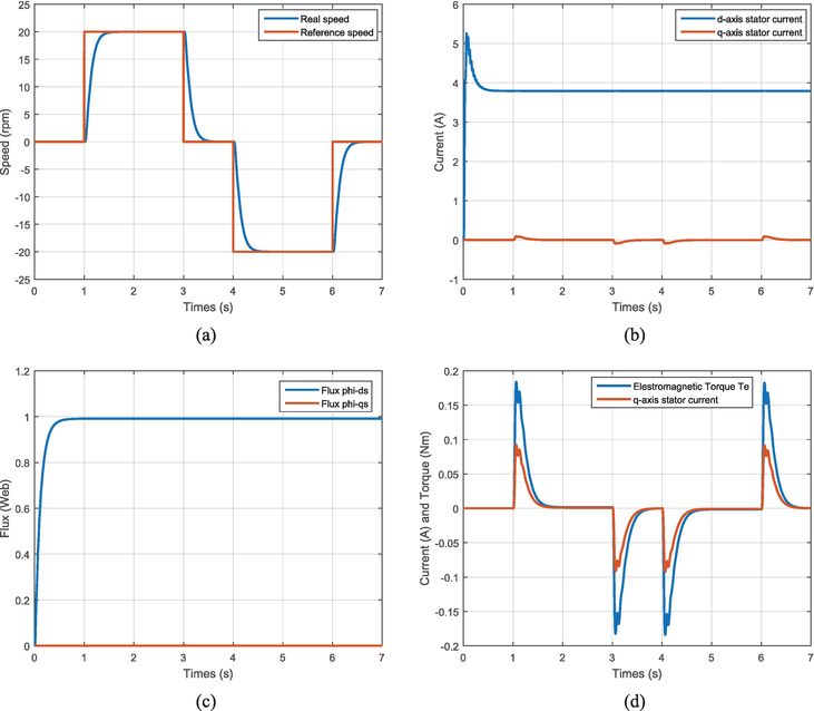
Figure 6.
Indirect stator flux-oriented controlled (ISFOC) induction motor drive for low speed.
5. Simultaneous estimation of the rotor speed and the rotor resistance
5.1 Description of the MRAS technique
The principle of estimation by this technique is based on the comparison of the outputs of two estimators from the knowledge of currents and stator voltages.
The first is called the reference model since it does not introduce the quantity to be estimated and the second is the adjustable one. The error between these two models drives an adaptation mechanism that updates the parameters of the adjustable model to make them converge to the real parameters [11, 12]. Figure 7 shows the basic block diagram of the MRAS method.
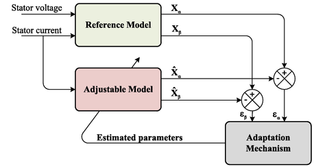
Figure 7.
The block diagram of the MRAS technique.
5.2 Simultaneous speed and rotor resistance estimation
For the estimation of the speed and the rotor resistance, it is judicious to use a stationary reference frame (α,β). This transformation does not use the position of the rotor, which is estimated by the MRAS strategy [11, 13].
The stator voltages can be described by the equation:
The rotor voltages can be described by the equation:
With
By using Eqs. (28) and (29) are rewritten under the following new form:
where
According to Eqs. (28) and (29), is it possible to identify ω and Rr. Afterward, we look to illustrate the components of the stationary reference frame stator flux (
The suitable adaptation mechanism that generates the estimation of ω and Rr, for the adjustable model is driven by the error between the states of the two models given by Eq. (31). It is noticed well that the feedback block
Eq. (6) can be presented as following [11, 14]:
where W is the feedback block, which establishes the input of the linear block.
For the speed estimation.
Eqs. (31) and (32) constitute a nonlinear feedback system represented by Figure 8. Indeed, this system can be schematized by a linear block described by the transfer matrix
For the rotor resistance estimation.
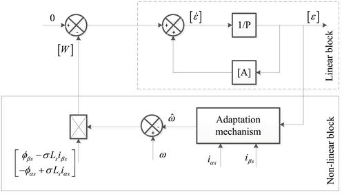
Figure 8.
Nonlinear feedback system for speed estimation.
Eqs. (31) and (32) constitute a nonlinear feedback system represented by Figure 9. Indeed, this system can be schematized by a linear block described by the transfer matrix
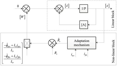
Figure 9.
Nonlinear feedback system for rotor resistance estimation.
The MRAS strategy consists to use the adaptation mechanism 1 to estimate ω. Subsequently, adaptation mechanism 2 is used to estimate Rr (Figure 10).
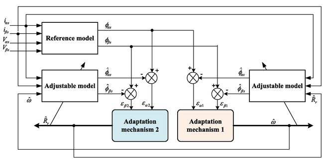
Figure 10.
Structure of the simultaneous speed and rotor resistance estimation by MRAS technique.
The asymptotic operation of the adaptation mechanism is fulfilled by a simplified condition, which is
With γ is a negative constant.
5.3 Speed adaptation mechanism
Adaptation mechanism 1 demonstrates that the estimated speed
where A1 and A2 are a nonlinear function of εα1, εβ1.
By using the expression of W, Eq. (33) is equivalent to
where K1 and K2 are called adaptation gains, which are constants and positive.
Eq. (34) is built around a PI regulator. Figure 11 represents the result of the synthesis of the speed regulator [11, 14].
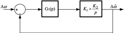
Figure 11.
Synthesis of the speed corrector.
To study the dynamic response of the estimated speed by the MRAS method, it is necessary to linearize the stator and the rotor equations around an operating point. Thus, the error variation ε is expressed as follows [11, 14]:
The transfer function representing the variation ratio Δε compared with
In a steady operation, one will have:
Then, by neglecting the effect of the slip pulses ωsl, the transfer function of G1(p) will be:
Hence, the transfer function of the direct chains is written:
The transfer function F(p) of the speed estimator is influenced by PI regulator coefficients K1 and K2, real speed, and induction motor parameters. To highlight the influence of the real speed on the stability of the estimator, the place of the zeros and the poles for the various values of ω are presented. When the rotor speed varies in the interval from 0 to 314 rad/s, the MRAS estimator poles location is presented in Figure 12. The results demonstrate that the variation speed does not affect the stability of the system.
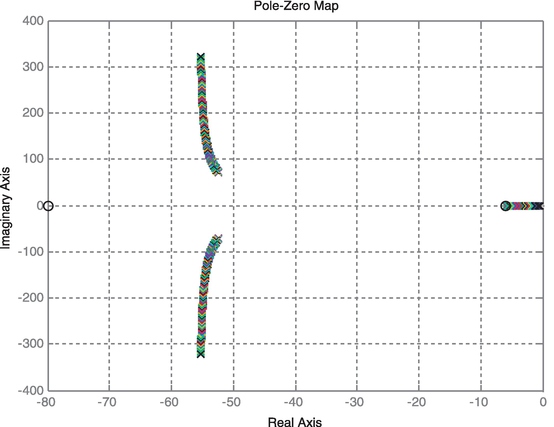
Figure 12.
Evolution of the MRAS estimator poles and zeros according to the speed.
5.4 Rotor resistance adaptation mechanism
Adaptation mechanism 2 demonstrates that the estimated rotor resistance is a function of the error [ε]. Then, it can be shown in the following form [11, 14]:
where A3 and A4 are a nonlinear function of εα2, εβ2.
Using the expression of W2, Eq. (33) is equivalent to:
where K3 and K4 are called adaptation gains, which are constant and positive.
Eq.(42) presents a transfer function that connects Δε with
In a steady operation, one will have:
The functional diagram in the closed loop of the rotor resistance estimation by the MRAS method is given in Figure 13.
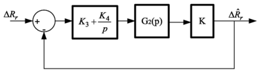
Figure 13.
Functional diagram of the rotor resistance estimation.
In this functional diagram, the expression of K is given by [14]:
Two complex poles (p1 and p2) are presented in the transfer function G2(p):
and
We note that the stability of the function is confirmed because the real part of the two complex poles p1 and p2 are negative. Furthermore, the application of a PI regulator allowed us to have a fast convergence and a null static error in the steady-state operation.
Figure 14 shows the layout of the root locations related to the transfer function G2(p) for 157 rad/s. It characterizes the dynamics of the control system. However, for this function, there are two poles and a zero, which are all located in the left half-plan of the complex plan. Moreover, the poles p1 and p2 are located at −5.94 ± 157j, which characterize the dynamics of the system. Then, to guarantee a good tracking performance and fast transient response, the zero placement of the PI regulator must be located on the real axis at −5.94. Thus, K3 must be taken of a rather large value and the ratio K4/K3 must be equal to the negative real part of the complex poles of the systems [16, 17] (K3 = 500 and K4/K3 = 5,94). This allows us to have an error in the rotor resistance that decreases the fast exponential form with time without oscillation.
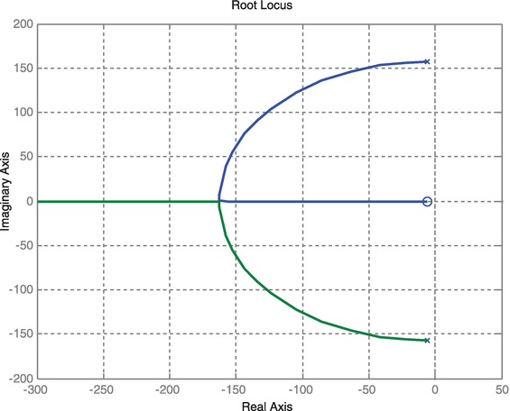
Figure 14.
Poles and zeros locations of G2(p).
Figure 15 shows the zero location of the controller PI (K4/K3) can be selected for the value of the rotor resistance. Otherwise, this figure presents the location of the poles of G2(p) with various values of Rr.
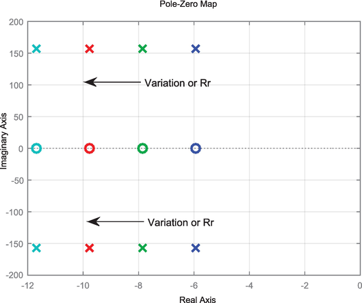
Figure 15.
Poles and zeros locations of G2(p) for different values of Rr.
5.5 Stator flux estimation
According to system Eq. (2), the two flux ϕαs and ϕβs are determined through the integration of the back EMF of the machine. The estimated flux is obtained by a pure integration and can cause significant problems, in particular, at the voltage shift (DC offset), at the uncertain parameters, and at low frequency due to the noise sensor. Thus, to overcome these problems, the pure integrator is changed with a low-pass filter (LPF) [18]. In this chapter, we propose to replace the pure integrator with a programmable cascaded low pass filter (PCLPF). This approach has already been proposed to control the IM without a mechanical sensor [19]. Indeed, a PCLPF includes a few blocks of these filters. Each block decreases the effect of the voltage shift (DC offset). In one PCLPF, their gains as well as their cut-off frequencies are given according to the stator frequency.
Therefore, two methods are proposed. A Modified Programmable Cascaded Low-Pass Filters (MPCLPF) present the first method, the estimate precision is improved by eliminating the gain in the calculation phase. The second method is called the Extended PCLPF (EPCLPF) [20], the estimator behavior is modified by the elimination of the gain G in the calculation phase and the extension low-pass filters stages (LPF stages). This method can be applied only to the area of a very low speed.
5.5.1 MPCLPF filter
The phase angle θs is calculated by dividing ϕβs(p) by ϕαs(p). Thus, G is a common factor in the two equations (ϕαs(p) and ϕβs(p)) and can be eliminated. (by simplification). However, it can be announced that:
H′(p), which is defined as the transfer function of MPCLPF is presented by Eq. (47).
5.5.2 Extended programmable cascaded low pass filter (EPCLPF)
As previously mentioned, the reduction of the continuous voltage shift (DC offset) is an effective means for sensorless control in the low-speed region [20]. As the output depends on the gain of the PCLPF, this list should be reduced. Here, it is necessary to take the relation between the amplitude of the gain and the order of the PCLPF into account. For a number of N LPF stages presented in Figure 16, the time-constant of the filters, the calculations of the gain and the transfer function are given below:
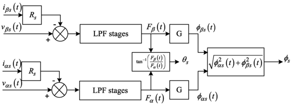
Figure 16.
Diagram of N floors of the programmable-low-flow filter.
By using Eqs. (51) and (52) becomes:
5.6 Simulation results
The simultaneous estimation algorithm by MRAS method has been simulated using Matlab-Simulink Software. Figure 17 shows the synoptic of simultaneous estimation in sensorless ISFOC IM drive based on MRAS scheme. However, the bloc diagram is made up of a PWM voltage source inverter, a coordinate translator, and a speed controller. A field orientation mechanism and an induction motor. Moreover, the gains of the PI current controller and IP gains speed controller are calculated and tuned at each sampling time, according to the new estimated rotor speed and rotor resistance.
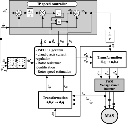
Figure 17.
Synoptic of ISFOC-oriented induction motor drive system with simultaneous estimation.
For the simulation of the proposed algorithm, we used a 3 kW induction motor knowing that these parameters are given in the Appendix. Furthermore, the sampling time for control algorithms computation and simultaneous estimation is used as 0.2 ms. Moreover, this sensorless ISFOC drive simulation was performed under various load and speed conditions. Thus, in Figure 18, at a speed of 1000 rpm and with a load torque, Rr was chosen to be equal to 1.55 Ω and increased by 50% from its initial value at t = 10 s. Knowing that the torque is applied with 10 Nm at t = 6 s and canceled at time t = 16 s. The two trajectories of estimated and reference rotor resistance coincide fairly well and a very good coincidence is reached. We also note that the error between the real and estimated rotor resistance is given in the Figure 18(b).
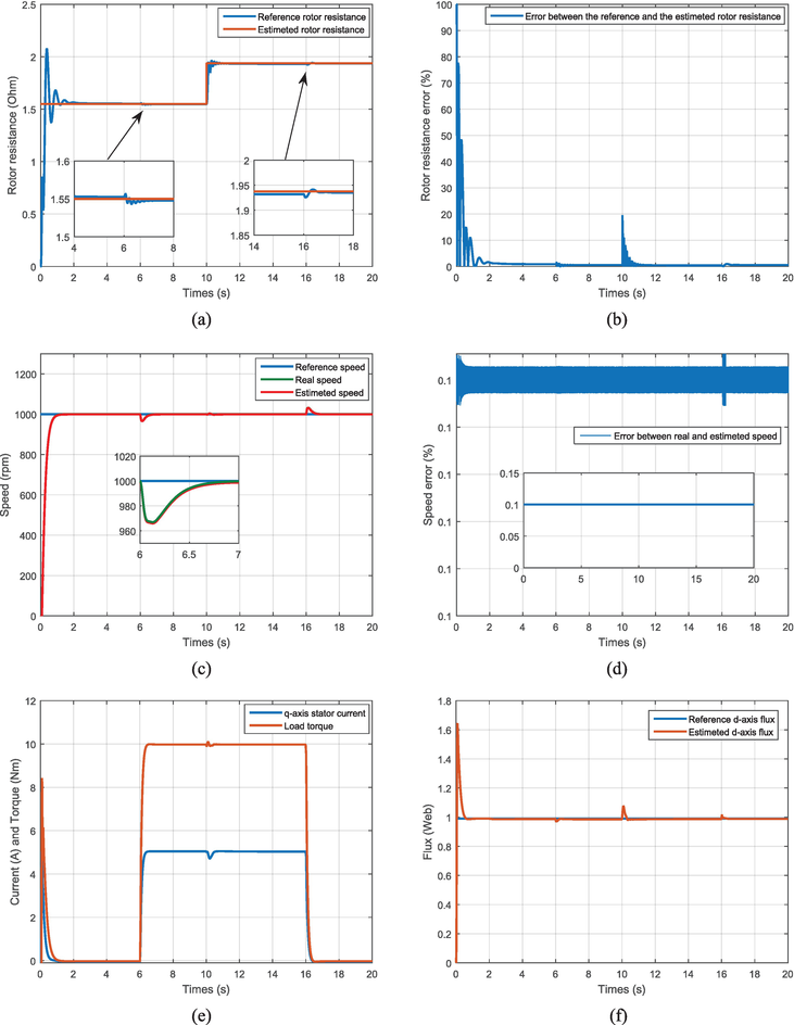
Figure 18.
Identification performance at nominal speed and load torque: (a) estimated and reference rotor resistance, (b) rotor resistance error, (c) reference speed, real speed, and estimated speed (d) estimated and reference flux, (e) iqs stator current and load torque, and (f) ϕds estimated and reference stator flux.
The increase of the rotor resistance agrees with an eventual heating of the rotor winding. The obtained result demonstrates that even if the rotor resistance changes, the proposed ISFOC procedure still gives a good estimate of this parameter. Figure 18(c) shows the simulation result of the reference, the estimated and the real speed using the IP controller. When the speed control changes from zero to 1000 rpm and the load torque applied and removed at t = 6 and 16 s, respectively, the error between the real and estimated rotor speed presented in Figure 18(d) is less than 0.15%. Furthermore, Figure 18(e) shows the measurement of the load torque and the q-axis stator current. The electromagnetic torque is estimated by the use of a stator current measurement. Moreover, the convergence of the estimated size of ϕds stator flux to its reference is proved by the Figure 18(f).
To show the robustness of the indirect control by the orientation of the stator flux, we applied a low-speed reference with the inversion of the rotation direction (0tr/mn → 150 pm → −15 rpm).
However, the estimated rotor resistance, as shown in Figure 19(a), matches the actual rotor resistance of the machine with a low error (Figure 19(b)) and so we obtain a robust control performance. Furthermore, in Figure 19(a), the three trajectories of estimated, real and reference rotor speed coincide fairly well and a good coincidence is reached. The results show that the ISFOC has a good tracking performance even at low speeds.
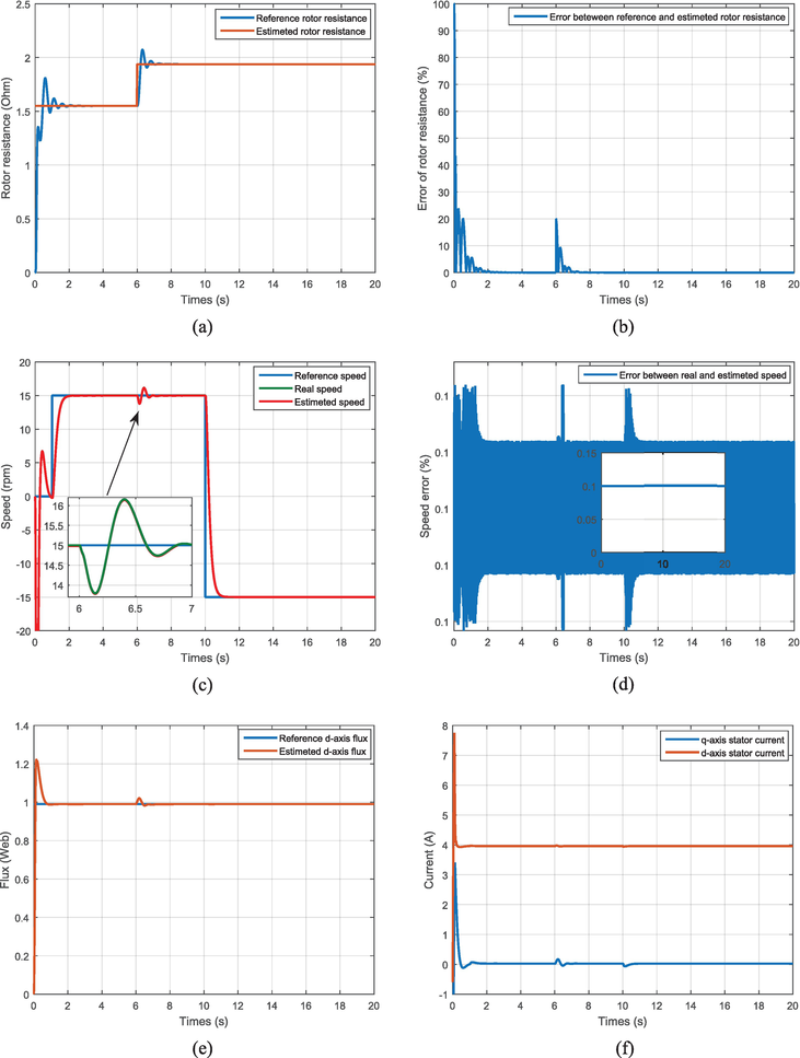
Figure 19.
Identification performance at nominal speed and load torque: (a) estimated and reference rotor resistance, (b) rotor resistance error, (c) reference speed, real speed, and estimated speed (d) estimated and reference flux, (e) iqs stator current and load torque, and (f) ϕds estimated and reference stator flux.
6. Experimental results
A prototype of the sensorless control with estimation of the rotor resistance of an asynchronous machine has been produced. As a result, experimental tests were carried out to validate the proposed algorithm and demonstrated the effectiveness and robustness of the MRAS technique. The experimental setup is composed of squirrel-cage IM a 3 kW, a voltage source inverter (VSI), pulse width modulation (PWM) signals to control the power modules generated by dSpace system, a hall-type sensors stator currents and stator voltages and a load generated through a magnetic power brake (Figure 20). Knowing that the experimentation has been achieved by using Matlab-Simulink and dSpace DS1104 real-time controller board.
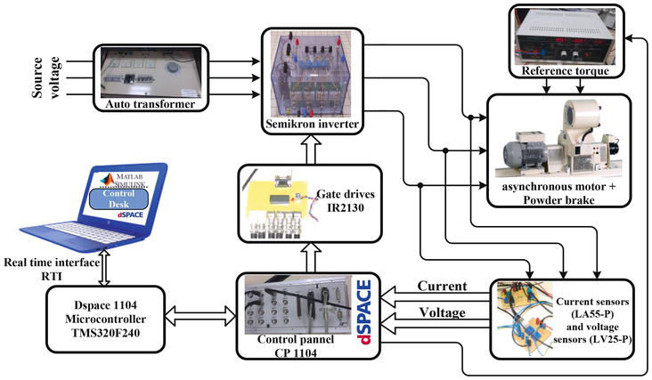
Figure 20.
Experimental setup.
Two cases will be presented for experimental validation:
First case: A speed reference of 15 rpm, and load torque (20 Nm) applied at t = 7 s and canceled at time t = 13 s.
Second case: A speed reference of 0 → 15 rpm → −15 rpm.
• The first case:
The experimental tests illustrated by Figure 21 (
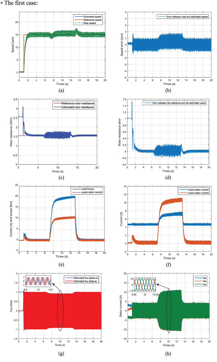
Figure 21.
Experimental results of step response (15 rpm) with load torque applied and removed at t = 7 s and 13 s, respectively.
• The second case:
In Figure 22, the sensorless ISFOC induction motor tests are carried out to show the effectiveness and robustness of the proposed scheme and the behaviors of the motor during speed transients. In Figure 22(a), the speed reversal test is performed and we note the convergence of the real and estimated speed toward its reference value. Therefore, Figure 22(b) shows that the error between the estimated and the real speed does not exceed 2 rpm in the steady state. Figure 22(c) shows that the convergence of the estimated value of rotor resistance
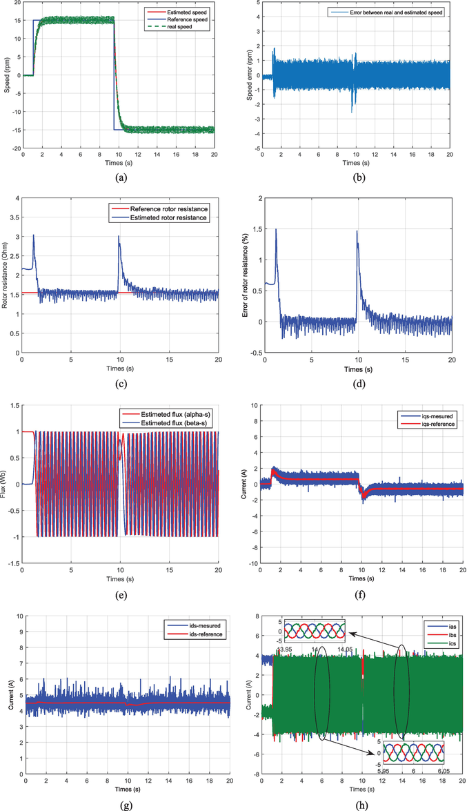
Figure 22.
Experimental results of step response ω = 15 rpm with inverting direction at the moment t = 9.5 s.
Finally, the Figure 22(h) proves the concordance of the stator currents
These results confirm the effectiveness, robustness, and good tracking performance of the ISFOC based on the MRAS scheme.
7. Conclusion
A simultaneous estimation of speed and rotor resistance in sensorless ISFOC induction motor drive based on the MRAS scheme has been presented. The variation of the rotor resistance is taken into account in order to guarantee the stability of the control system in all speed ranges with high-performance sensorless speed. The simultaneous estimation by the MRAS method is ensured by measuring the stator currents and voltages. Furthermore, the PI current and IP speed controller gains are online performed at each sampling time with the estimated value of the rotor resistance in order to provide optimal performance with guaranteed stability of the MRAS scheme.
From the simulation results, the simultaneous speed and rotor resistance estimation has proved the effectiveness and robustness of the sensorless ISFOC induction motor drive.
We have validated the online estimation for the rotor speed and the rotor resistance of an induction motor operating in an indirect stator field-oriented control system based on the MRAS method. The experimental results prove the robustness of this simultaneous estimation and the compliance with simulation results. The analyzed closed-loop stability of the proposed technique has also been proved through the Lyapunov stability theory. The experimental results show that the rotor resistance is sensitive to load variation. More importantly, the validity of the proposed sensorless ISFOC of the induction motor drive was proven by experiments for a wide range of speed and for a very low speed. More importantly, all experimental results confirm the good dynamic performances of the developed drive systems and show the validity of the suggested method. The obtained results show that the rotor resistance Rr is sensitive to load variation.
Nomenclature
d, q-axis stator voltage and current components
d, q-axis stator flux components
α, β-axis stator flux components
rotor and stator resistance
rotor and stator self-inductance
mutual inductance
number of pole pairs
synchronous and rotor angular speed
slip angular speed (ωs-ω)
electromagnetic and load torque
moment of inertia
friction constant
stator and rotor time constant
integral an proportional gain of the IP speed controller
integral and proportional gain of the PI current controller
total leakage constant
estimated and reference value
differential operator
List of motor specification and parameters: 380 V, 3 KW, 4 poles, 1430 rpm, Rs = 2.3 Ω; Rr = 1.55 Ω; Ls = Lr = 0.261 H; M = 0.245 H; f = 0.002 Nm s/rd; J = 0.03 kg m2.
References
- 1.
Jemli M, Boussak M, Goussa M, Kamoun MBA. Fail-safe implementation of indirect filed oriented controlled induction motor drive. Simulation Practice and Theory Journal. 2000; 8 :233-252 - 2.
Boldea I, Nasar SA. The Induction Machine Handbook. 1st ed. Boca Raton: CRC Press; 29 November 2001. p. 968. DOI: 10.1201/9781420042658 - 3.
Xing Y. A novel rotor resistance identification method for an indirect rotor flux-oriented controlled induction machine system. IEEE Transactions on Power Electronics. 2002; 17 :353-364 - 4.
Maiti S, Chakraborty C, Hori Y, Ta MC. Model reference adaptive controller based rotor resistance and speed estimation technique for vector controlled induction motor drive utilizing reactive power. IEEE Transactions on Industrial Electronics. 2008; 55 (2):594-601 - 5.
Akatsu K, Kawamura A. Online rotor resistance estimation using the transient state under the speed sensorless control of induction motor. IEEE Transactions on Power Electronics. 2000; 15 (3):553-560 - 6.
Miyashita I, Fujita H, Ohmori Y. Speed sensorless instantaneous vector control with identification of secondary resistance. In: Proc. IEEE IAS Annual Meeting. 1991. pp. E130-E135 - 7.
Jiang J, Holtz J. High dynamic speed sensorless ac drive with on-line model parameter tuning for steady-state accuracy. IEEE Transactions on Industrial Electronics. 1997; 44 :240-246 - 8.
Kubota H, Matsuse K. Speed sensorless field-oriented control of induction motor with rotor resistance adaptation. IEEE Transactions on Industry Applications. 1994; 30 :1219-1224 - 9.
Abdessamed R, Kadjoudi M. Modélisation des machines électriques. Presse de l’université de Batna Algerie. 1997 - 10.
Barret F. Régimes Transitoires des Machines Tournantes Électrique. Edition Eyrolls Paris: Collection des études et recherches d’électricité de France; 1982 - 11.
Agrebi Y, Triki MK, Y and Boussak, M. Rotor speed estimation for indirect stator flux oriented induction motor drive based on MRAS scheme. Journal of Electrical Systems. 2007; 3 (3):131-114 - 12.
Agrebi-Zorgani Y, Koubaa Y, Boussak M. MRAS state estimator for speed sensorless ISFOC induction motor drives with Luenberger load torque estimation. ISA Transactions. 2016; 61 :308-317 - 13.
Karlovský P, Linhart R, Lettl J. Sensorless determination of induction motor drive speed using MRAS method. In: Proceedings of the 8th International Conference on Electronics, Computers and Artificial Intelligence (ECAI). Ploiesti, Romania: IEEE Xplore; 2016. pp. 1-4 - 14.
Agrebi-Zorgani Y, Koubaa Y, Boussak M. Simultaneous estimation of speed and rotor resistance in sensorless ISFOC induction motor drive based on MRAS scheme. In: The XIX International Conference on Electrical Machines - ICEM 2010. Rome, Italy: IEEE; 2010. pp. 1-6 - 15.
Schauder C. Adaptive speed identification for vector control of induction motors without rotational transducers. IEEE Transactions on Industrial Applications. 1992; 28 (5):1054-1061 - 16.
Zaky MS. A stable adaptive flux observer for a very low speed sensorless induction motor drives insensitive to stator resistance variations. Ain Shams Engineering Journal, Production and Hosting by Elsevier. 2011; 2 (1):11-20 - 17.
Zaky MS. Stability analysis of speed and stator resistance estimators for sensorless induction motor drives. IEEE Transactions on Industrial Electronics. 2012; 59 (2):858-870 - 18.
Ghaderi A, Hanamoto T. Wide-speed-range sensorless vector control of synchronous reluctance motors based on extended programmable cascaded low-pass filters. IEEE Transactions on Industrial Electronics. 2011; 58 (6):2322-2333 - 19.
Ghaderi A, Hanamoto T, Teruo T. A novel sensorless low speed vector control for synchronous reluctance motors using a block pulse function-based parameter identification. Journal of power. Electronics. 2006; 6 (3):235-244 - 20.
Ghaderi A, Hanamoto T, Tsuji T. Very low speed sensorless vector control of synchronous reluctance motors with a novel startup scheme. In: IEEE Applied Power Electronics Conference and Exposition APEC. Anaheim, CA, USA. 25 Feburary-1 March 2007